Power to tail recursion

TLDR

We start with a simple recursive implementation of power function. And then keep improving it step by step to get to an iterative implementation. We will then see how tail recursion elimination can be done mechanically by a compiler. And leave with pondering about the future of programming languages.

Problem statement

Let’s start with a problem statement.

Write an algorithm that computes $x^{n}$ for a given $x$ and $n$ where $x$ is a real number and $n$ is a positive integer $> 0$ .

Journey through the solution space

Easy peasy.

x^{n} = {x, x^{n} * x^{n - 1}, if n = 1 . otherwise .

And simple Python implementation:

Listing 1. v0 - Naiive implementation

def power(x: int, n: int) -> int::
    if n == 1: return x
    else: return x * power(x, n - 1)

Not so fast. This is a recursive algorithm. It’s easy to understand, but it’s not very efficient. The time complexity of it is $O (n)$ . That’s because we’re doing n recursive calls.

Can we do better?

We can cut the recursive calls in half for each $n$ By observing that:

if n is even \to x^{n} = (x^{2})^{\frac{n}{2}}

Listing 2. v1 - Recursive implementation

def power(x: int, n: int) -> int:
    if n == 1: return x
    # if n is even
    if n % 2 == 0: return power(x * x, n // 2)
    # else n is odd
    else: return x * power(x, n - 1)

Now we’re doing only $l o g (n)$ recursive calls. That’s a big win. Time complexity of this algorithm is $O (l o g (n))$ assuming multiplication operation is $O (1)$ .

Figure 1. Comparing function call tree of v0 vs v1

How about space complexity? We’re doing $l o g (n)$ recursive calls, so we need to store $l o g (n)$ stack frames. So it is $O (l o g (n))$ as well. It is certainly better than $O (n)$ of v0.

But can we do better?

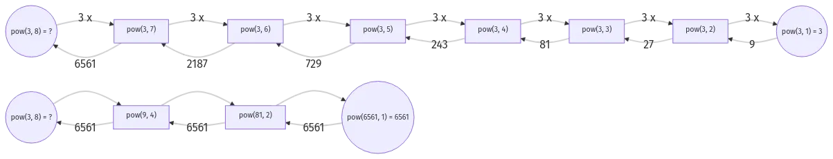
Let’s zoom into the function call tree of v1.

Figure 2. Function call tree of v1

We see that 6561 is being returned back through the call functions. We don’t need no stack frames for that.

The call stack is great when we need to store the state and return back to it later. Especially seen in backtracking algorithms. But in this case we don’t need to return back to the state. We just need to return the final value as the result.

Figure 3. It’s just iteration now

By viewing our previous function call tree as a loop, we can implement the same algorithm iteratively.

Listing 3. v2 - Iterative with a bit of recursion implementation

def power(x: int, n: int) -> int:
    while n > 1:
        if n % 2 == 0: # if n is even
            # return power(x * x, n // 2)
            x = x * x
            n = n // 2
        else: # else n is odd 1
            return x * power(x, n - 1)
    return x

1	Yes, I have pushed the `n is odd` case under the rug for now. We will get back to it soon.

Now we’re doing $l o g (n)$ iterations with $O (1)$ space complexity in the best case. Yay!

Let’s zoom back into Listing 2, “v1 - Recursive implementation” to see what was special in the case of $n$ being even?

Listing 4. Zooming into v1 implementation

def power(x: int, n: int) -> int:
    ...
    if n == 1: return x
    # if n is even
    if n % 2 == 0: return power(x * x, n / 2)
    ...

What was special is that, in the case of $n$ being even, the last "action" is a recursive call to the same function. And that is called tail recursion.

When recursive call is at the tail end of the function, it is called tail recursion.

Tail recursion is special because as we saw it can be easily converted to iteration. And this commonly known as tail call optimization or tail call elimination.

the base case is the exit condition of the loop
the recursive call is the loop itself
any variable transformations are the loop body

As you can see this conversion is totally mechanical when the conditions are met. And any optimizing compiler is able to do this.

But what if the conditions are not met?

Let’s zoom back into Listing 2, “v1 - Recursive implementation” to see what was special in the case of $n$ being odd?

Listing 5. Zooming again into v1 implementation

def power(x: int, n: int) -> int:
    ...
    if n == 1: return x
    # if n is even
    ...
    # else: n is odd
    else: return x * power(x, n - 1)

What’s special in the case of $n$ being odd is that, the last action is a multiplication. That’s pretty much the most basic requirement for tail call optimization. But no fear, we can find a way.

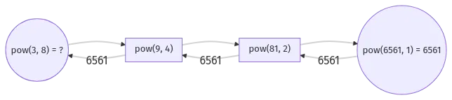
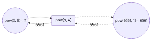
Let’s zoom into Figure 2, “Function call tree of v1”.

Figure 4. Zoom into function call tree of v1

Epiphany

We can see that pow(6561, 1) is a rewrite of the original function pow(3, 8). Actually every function call in the tree is a rewrite of the original function while simplifying to reach the base case.

In otherwords function parameters/arguments carry enough context to solve the original funtion.

Continuations

So in our problem how can we jam in the multiplication (x *) into the function parameters/arguments? We can literally jam it in by adding another parameter that passes it as a continuation (also can think of as a callback).

Listing 6. v3 - Iterative implementation with continuations

def power(x: int, n: int, cont: Callable[[int], int] = lambda x: x) -> int:
    if n == 1: return cont(x)
    # if n is even
    if n % 2 == 0:
        return power(
            x=x * x,
            n=n // 2,
            cont=cont
        )
    # else n is odd
    else:
        return power(
            x=x,
            n=n - 1,
            cont=lambda result: cont(x * result)
        )

Okay, let’s deconstruct what’s going on here.

We add a new parameter cont which is a function that takes an int and returns an int.
We add a default value for cont which is the identity function.
We call cont with the result of the function when we reach the base case.
For n is even we pass the continuation as is.
For n is odd we wrap the continuation with a new continuation that multiplies the result with x.

Since 5th point is the most interesting, diving a little deeper into it:

# Was else n is odd
else: return x * power(x, n - 1)

# Can be rewritten as
else:
    result = power(x, n -1) # result of the recursive call
    return x * result

# With continuation (just for this recursive step)
else: return power(x, n - 1, lambda result: x * result)

# Since the continuation of the current recusrive step
# needs to be followed by the continuation of the previous recursive step
# we need to compose the continuations
#
# continutaion                   continuation
# of current                     of previous
# recursive step                 recursive step
# ---------------               ----------------
#  (x * result)    followed by      cont
#
# which can be written as: cont(x * result)
#
else: return power(x, n - 1, lambda result: cont(x * result))

Small example just to make sure we’re on the same page:

Listing 7. v3 - Iterative implementation with continuations example

# to solve: power(x=3, n=6)
power(3, 6, lambda r: r)
# n is even
power(3 * 3, 6 // 2, lambda r: r)
# n is odd
power(9, 3 - 1, lambda result: (lambda r: r)(9 * result))
# n is even
power(9 * 9, 2 // 2, lambda result: (lambda r: r)(9 * result))
# n == 1
return (lambda result: (lambda r: r)(9 * result))(81)
= (lambda r: r)(9 * 81))
= 729

The final answer gets simplified beautifully to 729.

With Listing 6, “v3 - Iterative implementation with continuations” we have eliminated tail recursion once again. What’s cool is that the last transformation that we did can also be done mechanically by a compiler if they so wish.

But you are probably asking what did we really gain in Listing 6, “v3 - Iterative implementation with continuations” compared to Listing 3, “v2 - Iterative with a bit of recursion implementation”? We still have $O (n)$ space complexity in worst case because of the continuations.

Yes, we do. But we have gained something else. We have gained a hint of knowledge about continuations. Continuations are a powerful concept in programming languages that is worth exploring on it own. But we’re not going to do that here. We’re going to continue with our problem.

We can make one more observation in above Listing 7, “v3 - Iterative implementation with continuations example” to see if we can do better. We see that, we wait till the base case (n == 1) to simplify the result. Do we have to?

Let’s see how the base case looks like for another example.

# to solve: power(x=3, n=14)
...
# at n == 1
return (lambda r1: (lambda r2: (lambda r0: r0)(9 * r2))(81 * r1))(6561)
= (lambda r2: (lambda r0: r0)(9 * r2))(81 * 6561)
= (lambda r0: r0)(9 * 531441))
= 4782969

# ie. without continuation notation
= (9 * (81 * 6561)) 1
= 4782969

1	Notice the paranethesis that make the order of the operations explicit.

Because of the order of the operations we have to wait till the base case to simplify the result. But what if we can change the order of the operations? If we can do 9 * 81 first, then we can simplify the result at the recursive step itself.

And we can do that because we know that multiplication is associative.

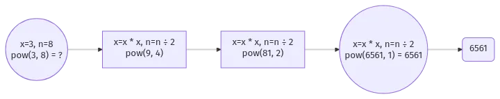
Armed with that knowledge let’s try to rewrite Listing 6, “v3 - Iterative implementation with continuations”. Instead of lazily accumulating continuations that will evaluate the result at the base case. Let’s eagerly evaluate the accumulations at the recursive step itself.

Listing 8. v4 - Tail recursive implementation with eager evaluation

def power(x: int, n: int, acc: int = 1) -> int:
    if n == 1:
        return acc * x
    # if n is even
    if n % 2 == 0:
        return power(x * x, n // 2, acc)
    # else n is odd
    else:
        return power(x, n - 1, acc * x)

Notice that we use 1 as the default value for acc instead of the identity function (lambda r: r). Because 1 is the identity element of the multiplication operation.

Side note

But what if the continuation (multiplication operation in this case) was not associative in Listing 6, “v3 - Iterative implementation with continuations”?

Then we would have to wait till the base case to evaluate the result. It would have essentially prevented us from transforming Listing 6, “v3 - Iterative implementation with continuations” to Listing 8, “v4 - Tail recursive implementation with eager evaluation”.

But fear not, you can read more about the fascinating idea of trampolines to approach this problem. The idea revolves around taking the continuation out of the stack and putting it in the heap.

Final implementation

Let’s put all the pieces together and convert Listing 8, “v4 - Tail recursive implementation with eager evaluation” to an iterative function.

To go from Listing 8, “v4 - Tail recursive implementation with eager evaluation” to Listing 9, “v5 - Final iterative implementation” we just need to remember the following:

the base case is the exit condition of the loop

the recursive call is the loop itself

any variable transformations are the loop body

Listing 9. v5 - Final iterative implementation

def power(x: int, n: int) -> int:
    acc = 1
    while n > 1:
        if n % 2 == 0: # if n is even
            # return power(x * x, n // 2, acc)
            x = x * x
            n = n // 2
        else: # else n is odd
            # return power(x, n - 1, acc * x)
            acc = acc * x
            n = n - 1
    return acc * x

We’re finally doing $l o g (n)$ iterations with $O (1)$ space complexity in the all cases. Yay!

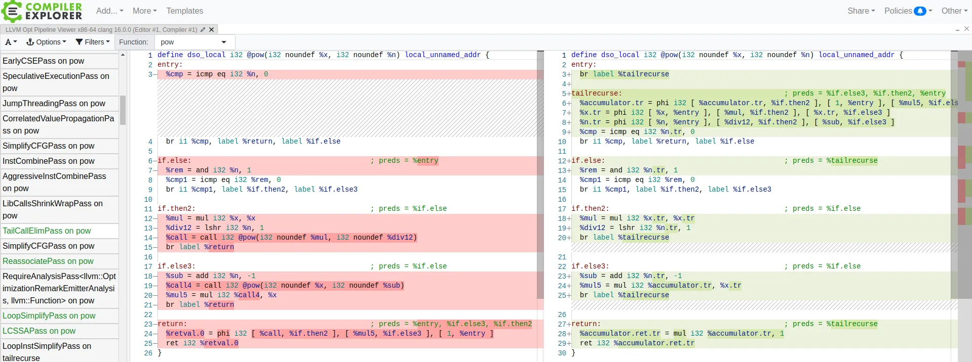
LLVM tail recursion elimination

What’s even cooler is that a sufficiently smart compiler can do this transformation for us, from Listing 2, “v1 - Recursive implementation” to Listing 9, “v5 - Final iterative implementation”.

Python doesn’t have tail call optimization. So we can’t see this transformation in action. But we can see it in action with C and clang compiler (-O3).

LLVM Pass: tailcallelim: Tail Call Elimination

This file transforms calls of the current function (self recursion) followed by a return instruction with a branch to the entry of the function, creating a loop. This pass also implements the following extensions to the basic algorithm:

Trivial instructions between the call and return do not prevent the transformation from taking place, though currently the analysis cannot support moving any really useful instructions (only dead ones).

This pass transforms functions that are prevented from being tail recursive by an associative expression to use an accumulator variable, thus compiling the typical naive factorial or fib implementation into efficient code.

TRE is performed if the function returns void, if the return returns the result returned by the call, or if the function returns a run-time constant on all exits from the function. It is possible, though unlikely, that the return returns something else (like constant 0), and can still be TRE’d. It can be TRE’d if all other return instructions in the function return the exact same value.

If it can prove that callees do not access their caller stack frame, they are marked as eligible for tail call elimination (by the code generator).

unsigned int pow(unsigned int x, unsigned int n) {
    if (n == 0) { return 1; }
    else if (n % 2 == 0) { return pow(x * x, n / 2); }
    else { return x * pow(x, n - 1); }
}

Figure 5. Tail recursion elimination in one of many LLVM IR optimization passes

The whole point of high level programming languages is to write programs that are easy to understand and reason about. And when we do that, we can let the compiler do the heavy lifting of optimizing the code for us.

Listing 1, “v0 - Naiive implementation” is obvious in its intentions but slow.
Listing 2, “v1 - Recursive implementation” is slightly less obvious but littler faster.
Listing 9, “v5 - Final iterative implementation” is fast but hides the intentions in lot of implementation details.

It would be awesome if the compiler can go from Listing 1, “v0 - Naiive implementation” to Listing 9, “v5 - Final iterative implementation”. But since it involves a bit of human ingenuity and knowledge of the problem domain, we will have to make do with compilers being able to transform Listing 2, “v1 - Recursive implementation” to Listing 9, “v5 - Final iterative implementation”.

Food for thought

Notice that even for clang to do the transformation, it had to know the properties of integer multiplication operation.

the fact that it is associative
the fact that it has an identity element

What if our function was matrix multiplication (matrix multiplication is also associative)? Can the compiler still do the transformation? Does the programming language have to provide a way to tell the compiler that the operation is associative?

Let’s close this note with food for thought.

If you are intrigued by that you should read "An axiomatic basis for computer programming" (C.A.R. Hoare. 1983).

In this paper an attempt is made to explore the logical foundations of computer programming by use of techniques which were first applied in the study of geometry and have later been extended to other branches of mathematics. This involves the elucidation of sets of axioms and rules of inference which can be used in proofs of the properties of computer programs. Examples are given of such axioms and rules, and a formal proof of a simple theorem is displayed. Finally, it is argued that important advantages, both theoretical and practical, may follow from a pursuance of these topics.